Start using Neural Networks not just for prediction, but for optimization.
In many engineering and scientific problems, we often deal with “black box” functions where the relationship between inputs and outputs is complex or expensive to compute (e.g., fluid dynamics simulations, finite element analysis). We want to find the input parameters that minimize (or maximize) some objective, but we can’t easily calculate gradients to guide us.
This is where Neural Networks as Surrogate Models come in.
The Concept
- Surrogate Modeling [1]: Train a Neural Network to approximate your expensive or unknown function $f(x)$ based on a set of sampled data points.
Why this works: The Universal Approximation Theorem guarantees that a feed-forward network with even a single hidden layer (and enough neurons) can approximate any continuous function to an arbitrary degree of accuracy. This massive theoretical flexibility is what allows us to confidently swap out complex physics simulations for a Neural Network.
- Differentiability: Unlike the black box function, a Neural Network is fully differentiable.
- Optimization: Once trained, we freeze the network’s weights. We then treat the input $x$ as the trainable parameter. By backpropagating the loss purely with respect to the input, we can use gradient descent to find the optimal $x$ that minimizes the output $y$.
Deep Dive: How Neural Networks Approximate Any Function
Before looking at the code, it is worth understanding why a Neural Network can mimic your physics equation or simulation. This property is known as the Universal Approximation Theorem [2].
1. The Single Neuron
A single neuron computes a weighted sum of inputs followed by a non-linear activation:
$$ y = \sigma(w \cdot x + b) $$
If we use a Tanh or Sigmoid activation, this looks like a smooth “step” or “S-curve”. It essentially splits the space into two: high values and low values. A single neuron is limited; it can only represent simple linear decisions (or a single step).
2. One Hidden Layer (The “Width” Argument)
The magic happens when we sum these neurons together. $$ F(x) = \sum_{i=1}^{N} v_i \cdot \sigma(w_i \cdot x + b_i) $$
Imagine you want to build a complex curvy shape using LEGO blocks.
- Each neuron is a single block (a simple bump or step).
- By adding enough neurons ($N \to \infty$) and scaling them ($v_i$), you can construct any continuous function to arbitrary precision.
- One neuron handles the “up” slope, another handles the “down” slope, and together they make a hill. Add more, and you can model mountains, valleys, or parabolas.
Theorem: A feed-forward network with a single hidden layer containing a finite number of neurons can approximate continuous functions on compact subsets (i.e., bounded ranges) of $\mathbb{R}^n$.
3. Two Hidden Layers (The “Depth” Argument)
If one layer is enough, why do we use deep networks? While one layer can do it, it might require an exponential number of neurons to fit complex functions (e.g., a function that oscillates wildly).
- Layer 1 learns simple features (edges, lines).
- Layer 2 combines those lines into shapes (squares, circles).
- Layer 3 combines shapes into objects.
By composing functions ($f(g(x))$), deep networks can represent complex hierarchies efficiently with far fewer total neurons than a massive single layer. This hierarchical structure is why deep networks generalize so well to unseen data (like our data gap test below).
Example: Minimizing a Parabola
Let’s demonstrate this with a trivial example so the mechanics are clear.
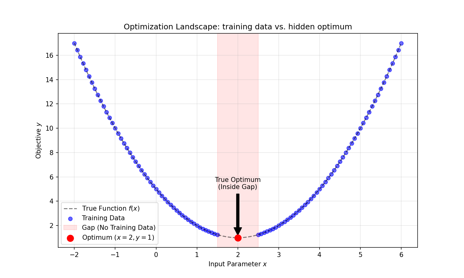
Suppose we want to minimize the function: $$ y = (x - 2)^2 + 1 $$
We know the minimum is at $x=2$ where $y=1$. But let’s pretend we don’t know the analytical form. We only have data samples.
Generalization Test
To make this more realistic, we will:
- Split Data: create a training set and a testing set.
- Create a Gap: Explicitly exclude the region around the optimum ($x \in [1.5, 2.5]$) from the training data. This forces the Neural Network to interpolate the shape of the function to find the minimum, rather than just memorizing a data point near $x=2$.
1. Generating Data with a Gap
First, we define our ground truth function $y = (x-2)^2 + 1$. Critically, we create a training dataset that excludes the region around the optimum ($x \in [1.5, 2.5]$). This tests if the model can generalize/interpolate rather than just memorizing.
import torch
import torch.nn as nn
import torch.optim as optim
import numpy as np

# A. The Ground Truth Function (The "Black Box")
def ground_truth(x):
    return (x - 2)**2 + 1

# B. Generate Data with a GAP at the optimum
# Optimum is at x=2. We exclude [1.5, 2.5] from training.
# Training data: [-2, 1.5] U [2.5, 6]
x_part1 = torch.linspace(-2, 1.5, 100)
x_part2 = torch.linspace(2.5, 6, 100)
X_train = torch.cat([x_part1, x_part2]).view(-1, 1)
y_train = ground_truth(X_train)

print(f"Training samples: {len(X_train)}")
print(f"The optimum (x=2) is explicitly REMOVED from training data.")
2. Defining the Surrogate Model
We use a simple Feed-Forward Neural Network. We choose Tanh activations because they produce smooth, continuous derivatives, which are better for gradient-based optimization than the piecewise-linear ReLU.
class SurrogateModel(nn.Module):
    def __init__(self):
        super().__init__()
        self.net = nn.Sequential(
            nn.Linear(1, 64),
            nn.Tanh(), # Tanh approximates smooth curves better than ReLU
            nn.Linear(64, 64),
            nn.Tanh(),
            nn.Linear(64, 1)
        )

    def forward(self, x):
        return self.net(x)

model = SurrogateModel()
3. Training the Model
We train the model using standard Supervised Learning to minimize Mean Squared Error (MSE). At this stage, we are just teaching the network to mimic the available data.
optimizer_model = optim.Adam(model.parameters(), lr=0.01)
criterion = nn.MSELoss()

print("Training Surrogate Model...")
for epoch in range(1000):
    optimizer_model.zero_grad()
    prediction = model(X_train)
    loss = criterion(prediction, y_train)
    loss.backward()
    optimizer_model.step()

print("Surrogate trained!")
4. Parametric Optimization (The Magic Step)
Now for the core concept. We freeze the model weights and creating a new trainable parameter param_x. We then run gradient descent on param_x to find the input that minimizes the output of the network.
# Start with a random guess far from the optimum
param_x = torch.tensor([0.0], requires_grad=True)

# Define an optimizer for the INPUT PARAMETER 'x', not the model weights
optimizer_param = optim.Adam([param_x], lr=0.1)

print(f"Initial Guess: x = {param_x.item()}")
print("Optimizing 'x' to find minimum...")

for step in range(100):
    optimizer_param.zero_grad()

    # Pass our parameter through the FROZEN surrogate
    # We want to minimize y, so 'loss' is just the output y itself
    pred_y = model(param_x.view(1, 1))

    # Backpropagate to get gradient dy/dx
    pred_y.backward()

    # Update x to move "downhill"
    optimizer_param.step()

    if step % 20 == 0:
        print(f"Step {step}: x_est = {param_x.item():.4f}")

print(f"\nFinal Result:")
print(f"Estimated x_min: {param_x.item():.4f}")
print(f"True x_min: 2.0000")
Even though the network never saw data points between $1.5$ and $2.5$, it successfully learned the parabolic curve and guided the optimization to the correct minimum at $x \approx 2.0$.
Note: You might see a result like
1.98or2.05instead of exactly2.0. This difference arises because the model is interpolating across the gap. Theoretically, infinite curves could fit the training data; the Neural Network picks the “smoothest” one, which is usually very close to, but not always exactly, the true function in the missing region.
Multiple Dimensions: Rosenbrock Function
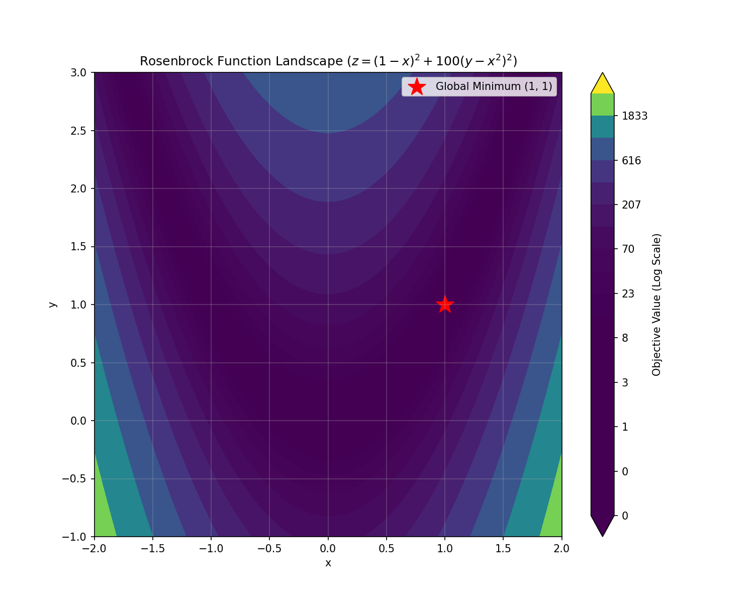
Let’s try something harder: the Rosenbrock function (often called the “banana function”). It’s a non-convex function used as a performance test problem for optimization algorithms.
$$ f(x, y) = (1 - x)^2 + 100(y - x^2)^2 $$
The global minimum is inside a long, narrow, parabolic shaped flat valley at $(x, y) = (1, 1)$. To find it, our Neural Network must navigate this valley.
Normalization is Key
For functions with large values (the Rosenbrock term $100(y-x^2)^2$ explodes easily), input/output normalization is crucial for the Neural Network to learn effectively.
1. The Challenge of Scale
The Rosenbrock function has terms that explode quickly (the $100(y-x^2)^2$ part). Neural Networks hate inputs with vastly different magnitudes. To make this work, we must standard scale (normalize) our inputs and targets to have roughly zero mean and unit variance.
import torch
import torch.nn as nn
import torch.optim as optim

# A. Rosenbrock Function
def rosenbrock(x, y):
    return (1 - x)**2 + 100 * (y - x**2)**2

# B. Generate Data
num_points = 5000
# Random points in range [-2, 2] for x and [-1, 3] for y
x_vals = torch.rand(num_points, 1) * 4 - 2
y_vals = torch.rand(num_points, 1) * 4 - 1
inputs = torch.cat([x_vals, y_vals], dim=1)
targets = rosenbrock(inputs[:, 0], inputs[:, 1]).view(-1, 1)

# C. Standardize Data (Critical for Convergence!)
input_mean, input_std = inputs.mean(dim=0), inputs.std(dim=0)
target_mean, target_std = targets.mean(), targets.std()

inputs_norm = (inputs - input_mean) / input_std
targets_norm = (targets - target_mean) / target_std
2. A Deeper Model
For this 2D non-convex problem, we use a slightly deeper network (3 hidden layers) to capture the complex “valley” shape.
model = nn.Sequential(
    nn.Linear(2, 64), nn.Tanh(),
    nn.Linear(64, 64), nn.Tanh(),
    nn.Linear(64, 64), nn.Tanh(),
    nn.Linear(64, 1)
)
3. Training
We train just like before, but notice we are training on the normalized data inputs_norm and targets_norm.
optimizer_model = optim.Adam(model.parameters(), lr=0.001)
loss_fn = nn.MSELoss()

print("Training...")
for epoch in range(2000):
    optimizer_model.zero_grad()
    loss = loss_fn(model(inputs_norm), targets_norm)
    loss.backward()
    optimizer_model.step()
4. Optimization in Generalized Space
This step requires care. Since our model thinks in “normalized units”, we must:
- Define our start point.
- Normalize that start point.
- Optimize in the normalized space.
- Denormalize the result to get the real-world answer.
# Start at random point (0, 3)
# 1 & 2. Normalize start point
start_norm = (torch.tensor([0.0, 3.0]) - input_mean) / input_std

# 3. Create trainable parameter in normalized space
param_norm = start_norm.clone().detach().requires_grad_(True)
opt_params = optim.Adam([param_norm], lr=0.05)

print("Optimizing...")
for step in range(200):
    opt_params.zero_grad()
    # Minimize the normalized output
    model(param_norm.unsqueeze(0)).backward()
    opt_params.step()

# 4. Denormalize to get real coordinates
final_res = param_norm * input_std + input_mean
print(f"Found Minimum: ({final_res[0].item():.4f}, {final_res[1].item():.4f})")
print(f"True Minimum:  (1.0000, 1.0000)")
This demonstrates that the generic “Surrogate + Gradient” method scales to multi-variable problems, provided you handle data scaling correctly.
Alternative Methods: Why Not Random Forests?
You might ask: Why not use a Random Forest or XGBoost? They are often state-of-the-art for regression.
We tried it. Here is what happens when you train a Random Forest on the same parabola data and try to find the minimum:
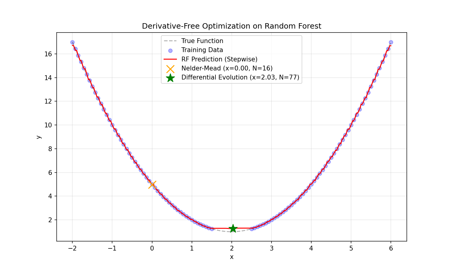
- Blocky Landscape: Tree-based models output “steps”. The function is not smooth.
- Gradient Descent Fails: Gradients are zero on the flat steps and undefined at the jumps. You simply cannot filter derivatives through a tree.
- Derivative-Free Methods?:
- Nelder-Mead (local search) failed in our test, getting stuck in a local flat region ($x \approx 0$).
- Genetic Algorithms (Differential Evolution) did find the minimum ($x \approx 2.03$), but it required 77 function evaluations for this simple 1D problem.
The Verdict: While Genetic Algorithms can optimize non-differentiable surrogates (like Random Forests), they suffer from the Curse of Dimensionality. For a 100-dimensional engineering problem, a Genetic Algorithm might need $100,000+$ evaluations. A Neural Network with gradients can solve it in a fraction of the steps.
Comparative Analysis: Random Forest vs. Neural Network
| Integration Feature | Random Forest (Tree-Based) | Neural Network (Differentiable) |
|---|---|---|
| Surface Smoothness | Step-wise / Blocky (Piecewise constant) | Smooth (Continuous derivatives) |
| Gradient Optimization | Gradients are 0 or undefined | Backpropagation gives exact direction |
| Optimization Method | Genetic Algorithms / Nelder-Mead | Gradient Descent (LBFGS / Adam) |
| Iterations | ~77 evaluations | Instantaneous gradient Step |
| Scalability | Poor (Curse of Dimensionality for search) | High (Gradients guide high-dim search efficiently) |
Conclusion
We explored two examples of using Neural Networks as differentiable surrogate models for optimization:
- 1D Parabola: A simple convex problem where the network successfully interpolated across a data gap. We showed that using Tanh activation provides a smoother, more robust approximation than ReLU without needing careful seed selection.
- 2D Rosenbrock: A complex non-convex problem. We demonstrated that data normalization (standard scaling) is critical for convergence when inputs and targets have vastly different magnitudes.
- Comparisons: We showed that traditional regression methods like Random Forests fail at this task because they produce piecewise constant “steps” with zero gradients. While Derivative-Free methods (Genetic Algorithms) can optimize these trees, they require significantly more function evaluations (77 vs. instantaneous) compared to the efficient gradient-based guidance provided by a Neural Network.
By treating the Neural Network not just as a predictor, but as a fully differentiable equation, we unlock the power of gradient-based optimization for any “black box” problem.
Summary
Using Neural Networks for parametric optimization is a powerful technique when:
- Gradients are unavailable: The original system is a “black box” simulation.
- Function evaluation is expensive: You can train the surrogate once and run optimization on it instantly.
- High-dimensional design space: NNs scale reasonably well to higher dimensions compared to grid search.
By combining the Universal Approximation capabilities of Neural Networks with the Automatic Differentiation of frameworks like PyTorch, we can solve complex engineering design problems that were previously intractable.
References
- Forrester, A., Sobester, A., & Keane, A. (2008). Engineering design via surrogate modelling: a practical guide. John Wiley & Sons.
- Hornik, K., Stinchcombe, M., & White, H. (1989). “Multilayer feedforward networks are universal approximators.” Neural Networks, 2(5), 359-366.